


My first post on this subject remarked on the number of scientists who assert that late 20th century global warming cannot have been driven by the sun because solar activity was not trending upwards after 1950, even though it remained at peak levels. To follow up, I asked a dozen of these scientists whether solar activity has to KEEP going up to cause warming?

Wouldn’t that be like saying you can’t heat a pot of water by turning the flame to maximum and leaving it there, that you have to turn the heat up gradually to get warming?
My email suggested that these scientists (more than half of whom are solar scientists) must be implicitly assuming that by 1980 or so, ocean temperatures had already equilibrated to the 20th century’s high level of solar activity. Then they would be right. Continued forcing at the same average level would not cause any additional warming and any fall off in forcing would have a cooling effect. But without this assumption-if equilibrium had not yet been reached-then continued high levels of solar activity would cause continued warming.
Pretty basic, but none of these folks had even mentioned equilibration. If they were indeed assuming that equilibrium had been reached, and this was the grounds on which they were dismissing a solar explanation for late 20th century warming, then I urged that this assumption needed to be made explicit, and the arguments for it laid out.
I have received a half dozen responses so far, all of them very gracious and quite interesting. The short answer is yes, respondents are for the most part defending (and hence at least implicitly acknowledging) the assumption that equilibration is rapid and should have been reached prior to the most recent warming. So that’s good. We can start talking about the actual grounds on which so many scientists are dismissing a solar explanation.
Do their arguments for rapid equilibration hold up? Here the short answer is no, and you might be surprised to learn who pulled out all the stops to demolish the rapid equilibration theory.
From “almost immediately” to “20 years”
That is the range of estimates I have been getting for the time it takes the ocean temperature gradient to equilibrate in response to a change in forcing. Prima facie, this seems awfully fast, given how the planet spent the last 300+ years emerging from the Little Ice Age. Even in the bottom of the little freezer there were never more than 20 years of “stored cold”? What is their evidence?
First up is Mike Lockwood, Professor of Space Environment Physics at the University of Reading. Here is the quote from Mike Lockwood and Claus Frohlich that I was responding to (from their 2007 paper, “Recent oppositely directed trends in solar climate forcings and the global mean surface air temperature”):
There is considerable evidence for solar influence on the Earth’s pre-industrial climate and the Sun may well have been a factor in post-industrial climate change in the first half of the last century. Here we show that over the past 20 years, all the trends in the Sun that could have had an influence on the Earth’s climate have been in the opposite direction to that required to explain the observed rise in global mean temperatures.
The estimate in this paper is that solar activity peaked in 1985. Would that really mean the next decade of near-peak solar activity couldn’t cause warming? Surely they were assuming that equilibrium temperatures had already been reached. Here is the main part of Mike’s response:
Hi Alec,
Thank you for your e-mail and you raise what I agree is a very interesting and complex point. In the case of myself and Claus Froehlich, we did address this issue in a follow-up to the paper of ours that you cite, and I attach that paper.
One has to remember that two parts of the same body can be in good thermal contact but not had time to reach an equilibrium. For example I could take a blow torch to one panel of the hull of a ship and make it glow red hot but I don’t have to make the whole ship glow red hot to get the one panel hot. The point is that the time constant to heat something up depends on its thermal heat capacity and that of one panel is much less than that of the whole ship so I can heat it up and cool it down without an detectable effect on the rest of the ship. Global warming is rather like this. We are concerned with the temperature of the Earth’s surface air temperature which is a layer with a tiny thermal heat capacity and time constant compared to the deep oceans. So the surface can heat up without the deep oceans responding. So no we don’t assume Earth surface is in an equilibrium with its oceans (because it isn’t).
So the deep oceans are not taking part in global warming and are not relevant but obviously the surface layer of the oceans is. The right question to ask is, “how deep into the oceans do centennial temperature variations penetrate so that we have to consider them to be part of the thermal time constant of the surface?” That sets the ‘effective’ heat capacity and time constant of the surface layer we are concerned about. We know there are phenomena like El-Nino/La Nina where deeper water upwells to influence the surface temperature. So what depth of ocean is relevant to century scale changes in GMAST [Global Mean Air Surface Temperature] and what smoothing time constant does this correspond to?
…In the attached paper, we cite a paper by Schwartz (2007) that discusses and quantifies the heat capacity of the oceans relevant to GMAST changes and so what the relevant response time constant is. It is a paper that has attracted some criticism but I think it is a good statement of the issues even if the numbers may not always be right. In a subsequent reply to comments he arrives at a time constant of 10 years. Almost all estimates have been in the 1-10 year range.
In the attached paper we looked at the effect of response time constants between 1-10 years and showed that they cannot be used to fit the solar data to the observed GMAST rise. Put simply. The peak solar activity in 1985 would have caused peak GMAST before 1995 if the solar change was the cause of the GMAST rise before 1985.
This is a significant update on Lockwood and Frohlich’s 2007 paper, where it was suggested that temperatures should have peaked when solar activity peaked. Now the lagged temperature response of the oceans is front and center, and Professor Lockwood is claiming that equilibrium comes quickly. When there is a change in forcing, the part of the ocean that does significant warming should be close to done with its temperature response within 10 years.
The Team springs into action, … on the side of a slow adjustment to equilibrium?
Professor Lockwood cites the short “time constant” estimated by Stephen Schwartz, adding that “almost all estimates have been in the 1-10 year range,” and indeed, it seems that rapid equilibration was a pretty popular view just a couple of years ago, until Schwartz came along and tied equilibration time to climate sensitivity. Schwartz 2007 is actually the beginning of the end for the rapid equilibration view. Behold the awesome number-crunching, theory-constructing power of The Team when their agenda is at stake.
The CO2 explanation for late 20th century warming depends on climate being highly sensitive to changes in radiative forcing. The direct warming effect of CO2 is known to be small, so it must be multiplied up by feedback effects (climate sensitivity) if it is to account for any significant temperature change. Schwartz shows that in a simple energy balance model, rapid equilibration implies a low climate sensitivity. Thus his estimate of a very short time constant was dangerously contrarian, prompting a mini-Manhattan Project from the consensus scientists, with the result that Schwartz’ short time constant estimate has now been quite thoroughly shredded, all on the basis of what appears to be perfectly good science.
Too bad nobody told our solar scientists that the rapid equilibrium theory has been hunted and sunk like the Bismarck. (“Good times, good times,” as Phil Hartman would say.)
Schwartz’ model
Schwartz’ 2007 paper introduced new way of estimating climate sensitivity. He showed that when the climate system is represented by the simplest possible energy balance model, the following relationship should hold:
τ = Cλ-1
where τ is the time constant of the climate system (a measure of time to equilibrium); C is the heat capacity of the system; and λ-1 is climate sensitivity
The intuition here is pretty simple (via Kirk-Davidoff 2009, section 1.1 ). A high climate sensitivity results when there are system feedbacks that block heat from escaping. This escape-blocking lengthens the time to equilibrium. Suppose there is a step-up in solar insolation. The more the heat inside the system is blocked from escaping, the more the heat content of the system has to rise before the outgoing longwave radiation will come into energy balance with the incoming shortwave, and this additional heat increase takes time.
Time to equilibrium will also be longer the larger the heat capacity of the system. The surface of the planet has to get hot enough to push enough longwave radiation through the atmosphere to balance the increase in sunlight. The more energy gets absorbed into the oceans, the longer it takes for the surface to reach that necessary temperature.
τ = Cλ-1 can be rewritten as λ-1 = τ /C, so all Schwartz needs are estimates for τ and C and he has an estimate for climate sensitivity.
Here too Schwartz keeps things as simple as possible. In estimating C, he treats the oceans as a single heat reservoir. Deeper ocean depths participate less in the absorbing and releasing of heat than shallower layers, but all are assumed to move directly together. There is no time-consuming process of heat transfer from upper layers to lower layers.
For the time constant, Schwartz assumes that changes in GMAST (the Global Mean Atmospheric Surface Temperature) can be regarded as Brownian motion, subject to Einstein’s Fluctuation Dissipation Theorem. In other words, he is assuming that GMAST is “subject to random perturbations,” but otherwise “behaves as a first-order Markov or autoregressive process, for which a quantity is assumed to decay to its mean value with time constant τ.”
To find τ, Schwartz examines the autocorrelation of the temperature time series and looks to see how long a lag there is before the autocorrelation stops being positive. This time to decorrelation is the time constant.
The Team’s critique
Given Schwartz’ time constant estimate of 4-6 years:
The resultant equilibrium climate sensitivity, 0.30 ± 0.14 K/(W m-2), corresponds to an equilibrium temperature increase for doubled CO2 of 1.1 ± 0.5 K. …
In contrast:
The present [IPCC 2007] estimate of Earth’s equilibrium climate sensitivity, expressed as the increase in global mean surface temperature for doubled CO2, is [2 to 4.5].
These results get critiqued by Foster, Annan, Schmidt and Mann on a variety of theoretical grounds (like the iffyness of the randomness assumption), but their main response is to apply Schwartz’ estimation scheme to runs of their own AR4 model under a variety of different forcing assumptions. Their model has a known climate sensitivity of 2.4, yet the sensitivity estimates produced by Schwartz’ scheme average well below even the low estimate that he got from the actual GMAST data, suggesting that an actual sensitivity substantially above 2.4 would still be consistent with Schwartz’ results.
Part of the discrepancy could be from Schwartz’ use of a lower heat capacity estimate than is used in the AR4 model, but Foster et al. judge that:
… the estimated time constants appear to be the greater problem with this analysis.
The AR4 model has known equilibration properties and “takes a number of decades to equilibrate after a change in external forcing,” yet when Schwartz’ method for estimating speed of equilibration is applied to model-generated data, it estimates the same minimal time constant as it does for GMAST:
Hence this time scale analysis method does not appear to correctly diagnose the properties of the model.
There’s more, but you get the gist. It’s not that Schwartz’ basic approach isn’t sensible. It’s just the hyper-simplification of his model that makes this first attempt unrealistic. Others have since made significant progress in adding realism, in particular, by treating the different ocean levels as separate heat reservoirs with a process of energy transport between them.
Daniel Kirk-Davidoff’s two heat-reservoir model
This is interesting stuff. Kirk-Davidoff finds that adding a second weakly coupled heat reservoir changes the behavior of the energy balance model dramatically. The first layer of the ocean responds quickly to any forcing, then over a much longer time period, this upper layer warms the next ocean layer until equilibrium is reached. This elaboration seems necessary as a matter of realism and it could well be taken further (by including further ocean depths, and by breaking the layers down into sub-layers).
K-D shows that when Schwartz’ method for estimating the time constant is applied to data generated by a two heat-reservoir model it latches onto the rapid temperature response of the upper ocean layer (at least when used with such a short time series as Schwartz employs). As a result, it shows a short time constant even when the coupled equilibration process is quite slow:
Thus, the low heat capacity of the surface layer, which would [be] quite irrelevant to the response of the model to slowly increasing climate forcing, tricks the analysis method into predicting a small decorrelation time scale, and a small climate sensitivity, because of the short length of the observed time series. Only with a longer time series would the long memory of the system be revealed.
K-D says the time series would have to be:
[S]everal times longer than a model would require to come to equilibrium with a step-change in forcing.
And how long is that? Here K-D graphs temperature equilibration in response to a step-up in solar insolation for a couple different model assumptions:
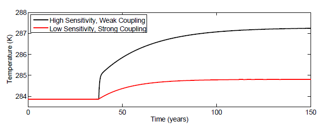

“Weak coupling” here refers to the two heat reservoir model. “Strong coupling” is the one reservoir model.
The initial jump up in surface temperatures in the two reservoir model corresponds to the rapid warming of the upper ocean layer, which in the particular model depicted here then warms the next ocean layer for another hundred plus years, with surface temperatures eventually settling down to a temperature increase more than twice the size of the initial spike.
This bit of realism changes everything. Consider the implications of the two heat reservoir model for the main item of correlative evidence that Schwartz put forward in support of his short time constant finding.
The short recovery time from volcanic cooling
Here is Schwartz’ summary of the volcanic evidence:
The view of a short time constant for climate change gains support also from records of widespread change in surface temperature following major volcanic eruptions. Such eruptions abruptly enhance planetary reflectance as a consequence of injection of light-scattering aerosol particles into the stratosphere. A cooling of global proportions in 1816 and 1817 followed the April, 1815, eruption of Mount Tambora in Indonesia. Snow fell in Maine, New Hampshire, Vermont and portions of Massachusetts and New York in June, 1816, and hard frosts were reported in July and August, and crop failures were widespread in North America and Europe – the so-called “year without a summer” (Stommel and Stommel, 1983). More importantly from the perspective of inferring the time constant of the system, recovery ensued in just a few years. From an analysis of the rate of recovery of global mean temperature to baseline conditions between a series of closely spaced volcanic eruptions between 1880 and 1920 Lindzen and Giannitsis [1998] argued that the time constant characterizing this recovery must be short; the range of time constants consistent with the observations was 2 to 7 years, with values at the lower end of the range being more compatible with the observations. A time constant of about 2.6 years is inferred from the transient climate sensitivity and system heat capacity determined by Boer et al. [2007] in coupled climate model simulations of GMST following the Mount Pinatubo eruption. Comparable estimates of the time constant have been inferred in similar analyses by others [e.g., Santer et al., 2001; Wigley et al., 2005].
All of which is just what one would expect from the two heat reservoir model. The top ocean layer responds quickly, first to the cooling effect of volcanic aerosols, then to the warming effect of the sun once the aerosols clear. But in the weakly coupled model, this rapid upper-layer response reveals very little about how quickly the full system equilibrates.
Gavin Schmidt weighs in
Gavin Schmidt recently had occasion to comment on the time to equilibrium:
Oceans have such a large heat capacity that it takes decades to hundreds of years for them to equilibrate to a new forcing.
This is not an unconsidered remark. Schmidt was one of co-authors of The Team’s response to Schwartz. Thus Mike Lockwood’s suggestion that “[a]lmost all estimates have been in the 1-10 year range,” is at the very least passé. The clearly increased realism of the two reservoir model makes it perfectly plausible that the actual speed of equilibration-especially in response to a long period forcing-could be quite slow.
Eventually, good total ocean heat content data will reveal near exact timing and magnitude for energy flows in and out of the oceans, allowing us to resolve which candidate forcings actually force, and how strongly. We can also look forward to enough sounding data to directly observe energy transfer between different ocean depths over time, revealing exactly how equilibration proceeds in response to forcing. But for now, time to equilibration would seem to be a wide open question.
Climate sensitivity
This also leaves climate sensitivity as an open question, at least as estimated by heat capacity and equilibration speed. Roy Spencer noted this in support of his more direct method of estimating climate sensitivity, holding that the utility of the fluctuation dissipation approach:
… is limited by sensitivity to the assumed heat capacity of the system [e.g., Kirk-Davidoff, 2009].
The simpler method we analyze here is to regress the TOA [Top Of Atmosphere] radiative variations against the temperature variations.
Solar warming is being improperly dismissed
For solar warming theory, the implications of equilibration speed being an open question are clear. We have a host of climatologists and solar scientists who have been dismissing a solar explanation for late 20th century warming on the strength of a short-time-to-equilibrium assumption that is not supported by the evidence. Thus a solar explanation remains viable and should be given much more attention, including much more weight in predictions of where global temperatures are headed.
If 20th century warming was caused primarily the 20th century’s 80 year grand maximum of solar activity then it was not caused by CO2, which must be relatively powerless: little able either to cause future warming, or to mitigate the global cooling that the present fall off in solar activity portends. The planet likely sits on the cusp of another Little Ice Age. If we unplug the modern world in an unscientific war against CO2 our grandchildren will not thank us.
(Addenda at bottom of Error Theory post.)